Taking as base the raw image dataset, without any additional information except for the pixels that make up their digital representations, each image was analyzed with a Convolutional Neural Network (CNN). For computers, images are nothing more than giant tables of numbers. Thus, a grayscale image of 100 × 100 pixels (100 high by 100 wide) can be seen as a table with 100 rows and 100 columns in which each cell contains a value that encodes the amount of white it contains. Black usually corresponds to the lowest value, 0; while the highest value is reserved for white. This higher value is arbitrary and depends on the desired color depth. It is usually common to encode up to 256 levels, requiring 1 byte to store each pixel (1 byte = 2 ^ 8 = 256). If instead of a grayscale image we have color images, each color is broken down into its components according to a color model. The RGB model, for example, decomposes each color additively into the amount of red (Red), green (Green), and blue (Blue), thus needing 3 values each between 0 and 256 to encode a color. This translates into storing a 3-dimensional point in each of those cells, or having 3 tables for each color component.
These tables or matrices are the inputs of the CNN. (Artificial) neural networks are machine learning systems loosely inspired by the biological neural networks present in the brains of animals. These systems “learn” to perform operations from examples, generally without being programmed with specific rules for each task. Internally, such a network is based on a set of connected units or nodes, called artificial neurons, that model the neurons of a biological brain. Each connection, like synapses in a biological brain, can transmit a signal to other neurons. An artificial neuron that receives a signal processes it and can signal neurons connected to it. The connections between neurons are weighted and the neurons are usually arranged in layers that connect sequentially (although this configuration allows for variations). The last layer is usually the output layer and is adjusted, in the case of supervised learning, to the number of cases to predict: cat vs. dog, person vs. animal, or multiple classes if necessary. Initially, the weights of the neurons are randomly distributed. When an input is processed, it passes through all the neurons according to how each one is activated, and upon reaching the output, the result is compared with the expected result -a difference known as loss-, adjusting the weights of the connections so that in the next iteration the output is more like expected; that is, the loss is minimized. With the sufficient number of iterations and training examples, the expected output and the output produced will be practically the same and the network will have learned a classification task, which is equivalent to knowing the set of specific weights of each connection, since the arrangement of layered neurons (the network architecture) and their activation functions do not change.
The peculiarity of CNN is that they perform convolution operations on images. These operations compress and reduce the images until they can be operated at the level of each layer of the network or even of independent neurons. In general, the number of neurons in the layers usually decreases from the input, reaches a minimum, and then grows back to the output layer. If our inputs are images of 100 × 100 RGB pixels and we want to classify cats vs. dogs, the input must be at least 3x100x100 and output 2. In the process, to achieve this condensation of information, convolutions are used to transform the space of the image in semantically equivalent spaces that maintain the necessary information to perform the classification. In general, the layer before the last one, that is, the layer that comes just before the end, is usually a vector that encodes the image in a much smaller space and maintains its semantic properties while allowing comparisons using operations of vector spaces on them. That is, if we look at that penultimate layer and represent it in a vector space, the distance between two images containing only dogs will be less than between an image containing a dog and another containing a cat.
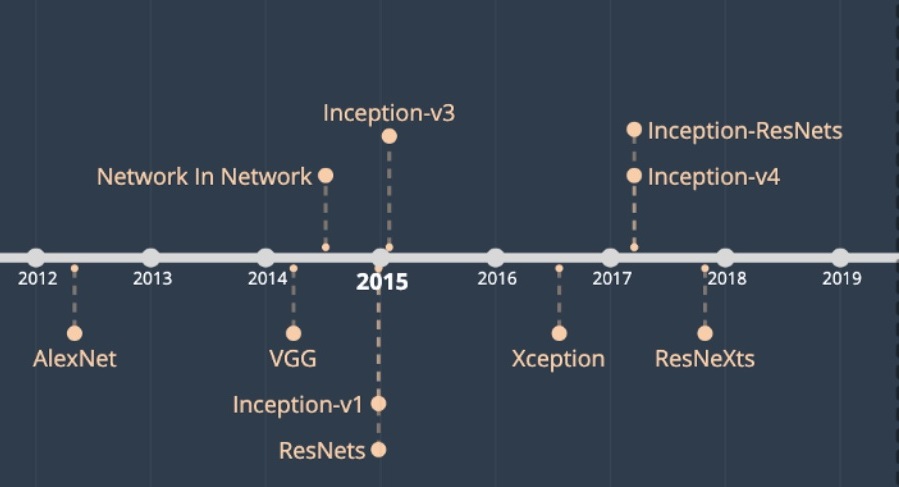
This information from the penultimate layer is what has been used to transform each image of the Barr X Inception CNN project into a vector that represents it. But instead of using as a goal a cat vs. dog classification task, version 3 of the trained Inception architecture has been used to classify more than 1,000 different categories on more than 1 million ImageNet 2012 images. In our case, at not needing the classification in those prefixed categories, we have used the information of the penultimate layer as a vector of numerical representation of each image that also maintains the expected properties of semantic similarity with respect to the operations of the vector space in which they are found.
However, the size of this vector (2,048) is too large to be represented in two-dimensional space. To solve this problem, a dimensionality reduction algorithm, specifically UMAP, has been applied to project the results of the analysis in a 2,048-dimensional space to a two-dimensional one that can be represented on a screen. UMAP is an algorithm for dimension reduction based on multiple learning techniques and ideas from topological data analysis. The first phase of the algorithm consists of the construction of a fuzzy topological representation. The second phase consists of optimizing the low dimensional representation to obtain a fuzzy topological representation as similar as possible according to a measurement borrowed from Information Theory (cross entropy). This allows us to transform a vector of 2,048 values into one of 2, allowing each image to be visually represented as a point in the vector space defined with UMAP, which in addition to being theoretically correct, has a strong mathematical basis.
The last step in the construction of our visual space is the identification of image clusters. Cluster detection has been performed with HDBSCAN, a refined version of the classic DBSCAN algorithm for unsupervised learning using hierarchy-arranged density measurements. Given a space, DBSCAN groups points that are very close together (points with many close neighbors), marking as points atypical points that are alone in low-density regions (whose closest neighbors are too far away). In this way, the algorithm is non-parametric, that is, it does not require any a priori information on the number of clusters to find, but will be able to identify an optimal number of clusters based on this idea of density.
In summary, the procedure for each image of an arbitrary size involves rescaling it and obtaining a vector representation according to the semantic relationships established by a CNN with Inception V3 architecture trained with the ImageNet 2012 dataset. This vector is reduced until obtaining a pair of coordinates that allow each image to be represented in a Cartesian space. Finally, these points are grouped into density clusters and the visualization is complete.
Recommeded quotation: De la Rosa, Javier. «Working with imagens anc CNN», in Barr X Inception CNN (dir. Nuria Rodríguez Ortega, 2020). Available at:http://barrxcnn.hdplus.es/working-with-iamges-and-cnn/ [date of access].